For sales leaders, tracking return on investment (ROI) in Excel is often the first step toward data-driven decision-making. Whether you're measuring the impact of a new sales tool or justifying headcount expansion, Excel provides an accessible starting point for ROI calculations.

While there are more sophisticated tools out there for complex sales operations, understanding how to calculate ROI in Excel gives you a foundation for tracking investment performance. 

This step-by-step guide will show you how to build basic ROI calculations in Excel that you can adapt for various sales initiatives. 

Basic ROI Formula

The standard calculation for ROI is as follows: 

                                                 ROI = (Net profit / Investment cost) x 100

Say you invest $5,000 in a new sales prospecting tool for your team. Over the next quarter, the increased efficiency helps your reps close an additional $15,000 in deals. The ROI calculation would look something like this:

                                                           (15,000 / 5,000) x 100 = 300%

This means that for every dollar spent on the prospecting tool, you generated $3 in additional sales, or a 300% return.

Of course, not every ROI calculation is this straightforward. Using Microsoft Excel will help you generate accurate data for more complex ROI calculations.

Setting Up an ROI Calculator in Excel: Step-by-Step Guide

Ready to build an ROI calculator in your Excel spreadsheets? Here’s a step-by-step look at the process. 

Step 1: Create an Excel Spreadsheet and Define Your Variables

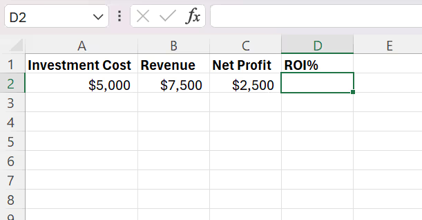
Start by creating a new Excel workbook. Create columns at the top of the sheet with the following labels: 

• Investment cost
• Revenue
• Net profit (Revenue - Investment)
• ROI% ((Net profit / Investment cost) x 100)

Step 2: Input Data

Next, input your data in the corresponding columns. 

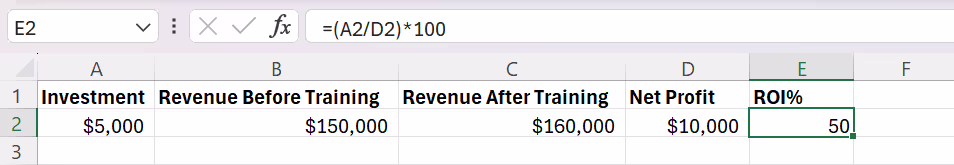
Say your team invested $5,000 in advanced sales training for your reps. The following quarter, this training generated an additional $7,500 in closed deals, resulting in $2,500 in net profit after accounting for the training cost.

At this point, the spreadsheet should look something like this: 

You can enter your net profit amount manually, or to speed things up, you can add the following calculation in cell C2: =B2-A2

Step 3: Use Excel Formulas to Calculate ROI

Once the correct data is in place, use Excel formulas to calculate your ROI automatically. An Excel formula performs a specific mathematical calculation in a target cell based on the data you’ve already provided.  

In this scenario, you’ll use the following formula: (Net profit / Investment cost) x 100

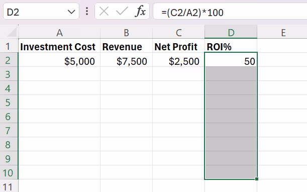
To calculate this, we’ll enter the following in cell D2: =(C2/A2)*100

Excel will calculate your ROI automatically. In this scenario, the ROI is 50%. Click and hold to select the D column. This will apply the calculation to all cells in that column when you add more rows of data. 

Step 4: Add Conditional Formatting for Quick Analysis

Excel’s conditional formatting feature makes it easy to categorize and assess your ROI metrics at a glance. With conditional formatting, you can color-code high and low ROI values to make them pop on the page. 

For example, you can use red to highlight cells with a negative ROI, while using green to highlight cells with a positive ROI. This makes it easier to visualize the financial impact of your business strategy. 

To add conditional formatting to your ROI spreadsheet, use the following steps: 

1. Select the cells to apply the conditional formatting to. In this case, you’ll apply conditional formatting to cells in the ROI% column. 
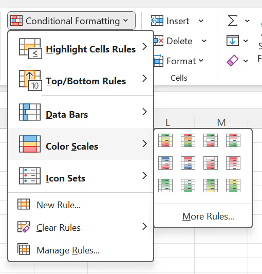
2. Select “Home” then “Conditional Formatting” from the menu.
3. Select the conditional formatting rule you’d like to use. 

There are several different formatting rules to choose from based on how you’d like to color-code your chart. 

For example, you can use “Highlight Cells Rules” or “Top/Bottom Rules” to highlight only ROI figures in a specific range or figures that are below or above a certain number. Use this strategy to pinpoint outliers in your ROI calculations and flag them for further analysis. 

Another option is to use the “Color Scales” tool to color-code all ROI figures in each column. This feature uses a red, yellow, and green color scale. 

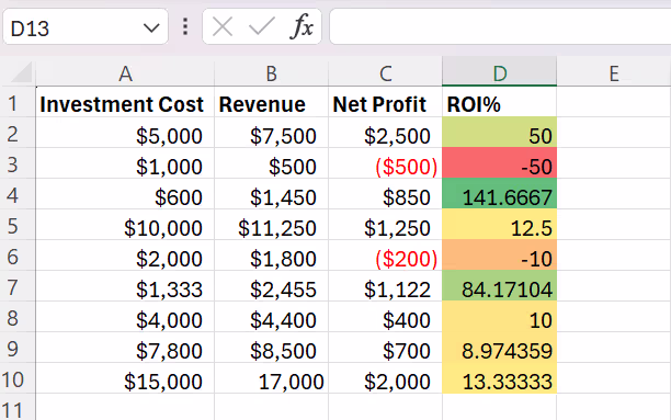
The intensity of the colors in each column will correlate with the numbers in each column. For example, extremely positive ROIs will be a deep green color, while negative ROIs will be a bright red, with moderate ROIs landing somewhere in the middle of the color spectrum. 

Step 5: Build a Dynamic ROI Calculator With Excel Functions

In many cases, your ROI calculations won’t be this straightforward. Implementing advanced Excel functions in your ROI spreadsheet will help you account for complexity and nuance in your calculations. 

Here are some additional functions you can use to create a dynamic ROI calculator in Excel. 

IF Function

The IF function generates a conditional output based on the values present in other cells. This function makes it easy to label and compare pieces of data in your ROI spreadsheet. 

For example, you might add an extra column to your spreadsheet to indicate whether each investment was profitable or unprofitable. Use the IF function to automatically display PROFITABLE for ROIs over a certain threshold and UNPROFITABLE for ROIs that do not meet this threshold. You can adjust the text to suit your needs. 

Here’s what this function looks like: 

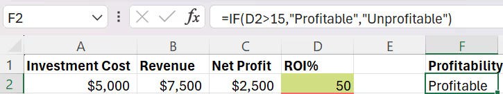
In this scenario, we’ve used 15% as the threshold for a profitable ROI. However, you can adjust this figure based on your industry and business model. 

SUM Function

The SUM function in Excel automatically calculates the sum of numerical values from specific cells. This function is helpful for calculating your organization’s total investment expenditures, profit, and ROI across a given time frame. 

Say you want to calculate the total ROI for investments within a given year. Enter =SUM, followed by the range of cells you want to add up. 

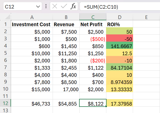
In this case, we used the SUM function for columns A, B, and C. To calculate the total ROI percentage, we used the formula =(C12/A12)*100 in column D12.

AVERAGE Function

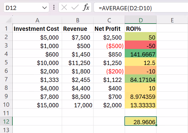
Excel’s AVERAGE function calculates the average of figures from selected cells. When tracking ROI, you can use this function to calculate average profits and ROIs over a select period of time. 

Say you've rolled out new sales productivity tools across different regional teams over the last year. After calculating the ROI for each regional rollout, use the =AVERAGE function to determine the average ROI across all regions. 

Your team can use this data to predict potential returns when expanding the tools to new territories and make informed decisions about future technology investments.

Dropdown Menus

Adding dropdown menus to your Excel spreadsheet is a simple but effective way to add more context to your ROI data. 

Say you’d like to categorize each row in your ROI spreadsheet based on the type of investment you’re making. Possible categories could include staffing, infrastructure, or technology. 

Follow these steps to create a dropdown menu: 

1. Select the cells where you want to apply a dropdown list. 
2. Select “Data” and then “Data Validation.” These options are found in the menu at the top of your screen. 

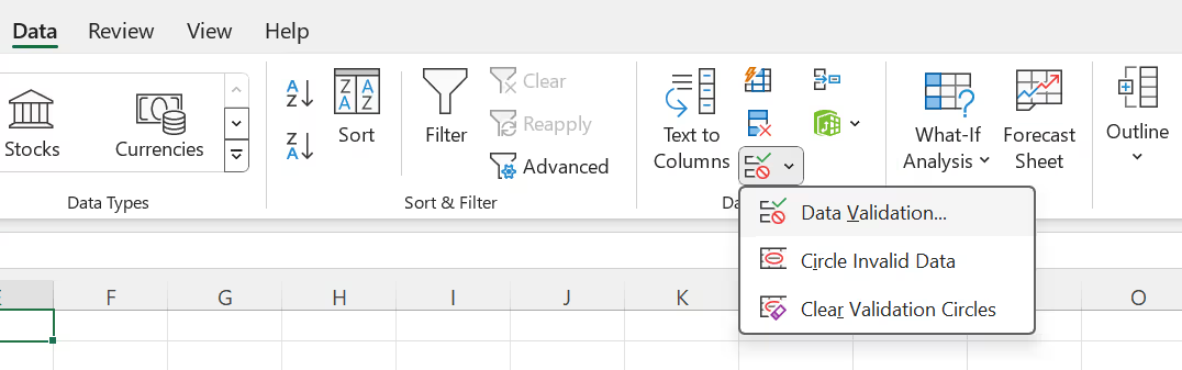
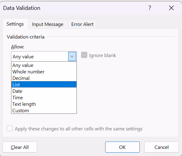
3. Select “Allow” to pull up the data validation menu. Select “List.” 

4. Enter your desired list options. In this case, we used “R&D,Staffing,Marketing,Infrastructure,Technology.” Do not add spaces between the list options. 

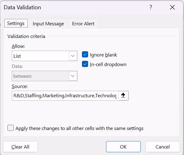
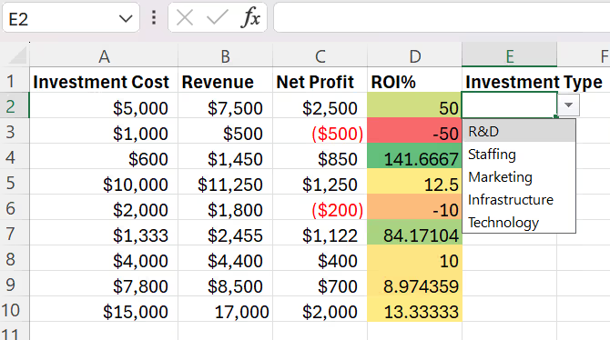
5. Select “OK” to confirm. When you click on the cells where the dropdown menu has been applied, you’ll be able to choose from your predetermined options. 

Example: Calculating ROI of a Sales Automation Platform 

Here's a look at ROI Excel calculations in action.

Say you've invested in a new sales automation platform for your team. This tool automates follow-up emails, meeting scheduling, and pipeline tracking to help your reps spend more time selling.

Calculating the ROI of this automation tool determines whether it's delivering value and helps inform future technology investments.

This ROI calculation involves the following components:

Investment: This is the cost of the automation platform, including implementation and licenses. In this case, the investment is $5,000.

Timeframe: Before performing the ROI calculations, you'll need to determine an appropriate timeframe to measure. For example, you might compare sales data from three months before and after implementing the automation tool.

Your chosen timeframe should be long enough to account for implementation and adoption. If you select a timeframe that's too short, you may miss the full impact of the automation on your sales process.

Revenue before automation: Add up the revenue from the designated period prior to implementing the tool. In this case, revenue before automation was $150,000 for three months.

Revenue after automation: Then, use the revenue from the three-month period after implementation to calculate your net profit. In this case, the revenue is $160,000, resulting in $10,000 of additional profit. While multiple factors can influence revenue growth, for this calculation, we can reasonably attribute this increase to the time saved through automation.

ROI calculation: With this example, the ROI calculation looks like this: 

                                                  (5,000 / 10,000) * 100 = 50% ROI

Analysis: In this situation, a 50% ROI indicates the automation tool is delivering solid returns. This suggests the investment is effectively helping reps focus more time on revenue-generating activities. The ROI could increase further as teams become more proficient with the tool and discover additional use cases.

The threshold for a good ROI varies based on your industry, the size of your organization, and the type of investment. For example, the median ROI for new software programs is very high at 278%, while investments in new staffing or infrastructure might not be as significant. 

From Excel Spreadsheets to Modern Solutions

While Excel has long been a go-to tool for basic calculations, it's not equipped to handle the complexities of fast-paced sales environments. Managing sales performance and tracking commissions becomes cumbersome and error-prone in static spreadsheets. Sales leaders need more than manual number-crunching — they need agile, data-driven insights that scale with their teams.

With real-time data, automated commission tracking, and advanced analytics, CaptivateIQ empowers you to accurately measure the ROI of your incentive strategies—all without the limitations of traditional spreadsheets.

Say goodbye to outdated tools, and let CaptivateIQ transform your sales strategy into a data-driven engine. Book a meeting today to get started!